📚 Attribution: The examples and explanations here are based on Appendix A (the PyTorch introduction) from Build a Large Language Model (From Scratch) by Sebastian Raschka, with the Python/PyTorch code ported to Rust/Candle. The diagrams are also adapted from the book.

This is a small guide for getting started with neural networks in Rust using Candle — a minimalist ML framework by Hugging Face. If you want to get hands-on with ML in Rust, this guide takes you from basic tensor operations to building and training a complete neural network.

Why Candle?

Candle is designed to be simple and easy to use. If you've used PyTorch before, many concepts will feel familiar:

• Tensors as the core data structure
• Similar operations for creating and manipulating tensors
• Automatic differentiation for gradients
• GPU support when you need it
• Pure Rust, no Python runtime needed

Another advantage is that Candle's API is intentionally similar to PyTorch, which makes porting code pretty straightforward.

Setting Up Candle

To get started with Candle, add it to your Cargo.toml file:

[dependencies]
candle-core = "0.9.1"
candle-nn = "0.9.1"
rand = "0.9.2"

• candle-core: Contains tensors and basic operations
• candle-nn: Provides neural network layers, optimizers, and loss functions
• rand: Used for shuffling data in the DataLoader

CPU vs GPU

By default, Candle works on CPU. If you want GPU support, you can enable CUDA features:

[dependencies]
candle-core = { version = "0.9.1", features = ["cuda"] }
candle-nn = { version = "0.9.1", features = ["cuda"] }

You'll need CUDA installed on your system for GPU support. All examples in this post use CPU, so that you can follow along on any machine.

Note: This guide uses Candle version 0.9.1. As Candle is actively developed, some APIs may change in future versions. Check the official documentation for the latest updates.

Understanding Tensors

Tensors represent a mathematical concept that generalizes vectors and matrices to potentially higher dimensions. In other words, tensors are mathematical objects that can be characterized by their order (or rank), which provides the number of dimensions.

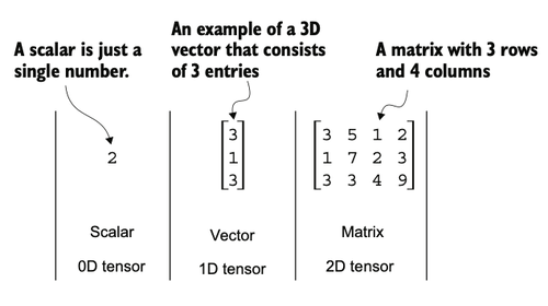
For example, a scalar (just a number) is a tensor of rank 0, a vector is a tensor of rank 1, and a matrix is a tensor of rank 2. A three-dimensional vector, which consists of three elements, is still a rank 1 tensor.

Tensors as Data Containers

From a computational perspective, tensors serve as data containers. They hold multidimensional data, where each dimension represents a different feature. Tensor libraries like Candle can create, manipulate, and compute with these arrays efficiently. In this context, a tensor library functions as an array library.

Candle tensors are similar to PyTorch tensors but built for Rust. They have several features that are important for deep learning:

• An automatic differentiation engine for computing gradients
• GPU support to speed up deep neural network training
• Efficient operations optimized for machine learning

Candle adopts a PyTorch-like API for its tensor operations, which makes it familiar if you've used PyTorch before.

Creating Tensors

As mentioned earlier, Candle tensors are data containers for array-like structures. A scalar is a zero-dimensional tensor (just a number), a vector is a one-dimensional tensor, and a matrix is a two-dimensional tensor. For higher dimensions, we refer to them as 3D tensors, 4D tensors, and so on.

We can create Candle tensors using the Tensor::new function:

use candle_core::{Tensor, Device};

fn main() -> Result<(), candle_core::Error> {
    let device = Device::Cpu;

    // Creates a zero-dimensional tensor (scalar)
    let tensor0d = Tensor::new(&[1u8], &device)?;

    // Creates a one-dimensional tensor (vector)
    let tensor1d = Tensor::new(&[1., 2., 3.], &device)?;

    // Creates a two-dimensional tensor (matrix)
    let tensor2d = Tensor::new(&[[1., 2.], [3., 4.]], &device)?;

    // Creates a three-dimensional tensor
    let tensor3d = Tensor::new(&[[[1., 2.], [3., 4.]], [[5., 6.], [7., 8.]]], &device)?;

    Ok(())
}

In Candle, we need to specify a device (CPU or GPU) when creating tensors. The ? operator handles potential errors that might occur during tensor creation.

Tensor Data Types

When creating tensors in Candle, the data type depends on what values you provide. We can check a tensor's data type using the .dtype() method:

let tensor1d = Tensor::new(&[1u8], &device)?;
println!("{:?}", tensor1d.dtype());

This prints:

U8

If we create tensors from floating-point numbers, Candle uses the type from Rust's default float literal, which is 64-bit:

let floatvec = Tensor::new(&[1.0, 2.0, 3.0], &device)?;
println!("{:?}", floatvec.dtype());

The output is:

F64

However, for deep learning, 32-bit floating-point precision is usually preferred. It offers sufficient precision for most tasks while consuming less memory and computational resources than 64-bit. GPU architectures are also optimized for 32-bit computations, which speeds up model training and inference.

Changing Data Types

You can change the precision using a tensor's to_dtype method. The following code demonstrates changing a tensor to 32-bit or 8-bit:

let tensor = Tensor::new(&[[[1., 2.], [3., 4.]]], &device)?;
println!("{:?}", tensor.dtype()); // F64

let tensor = tensor.to_dtype(DType::F32)?;
println!("{:?}", tensor.dtype()); // F32

let tensor = tensor.to_dtype(DType::U8)?;
println!("{:?}", tensor.dtype()); // U8

Candle supports various data types including F64, F32, U8, U32, and more. You can find them in the candle_core::DType enum.

Common Tensor Operations

Comprehensive coverage of all the different Candle tensor operations is not included in this post. However, we will cover the most relevant operations you'll need for building neural networks.

We've already seen how to create tensors using Tensor::new:

let tensor2d = Tensor::new(&[[1., 2., 3.], [4., 5., 6.]], &device)?;
println!("{}", tensor2d);

This prints:

[[1., 2., 3.],
 [4., 5., 6.]]
Tensor[[2, 3], f64]

Checking Tensor Shape

The .shape() method allows us to access the shape of a tensor:

println!("{:?}", tensor2d.shape());

The output is:

[2, 3]

This means the tensor has two rows and three columns.

Reshaping Tensors

To reshape the tensor into a 3 × 2 tensor, we can use the .reshape method:

println!("{}", tensor2d.reshape((3, 2))?);

This prints:

[[1., 2.],
 [3., 4.],
 [5., 6.]]
Tensor[[3, 2], f64]

Note that Candle's reshape requires the new shape to have the same total number of elements as the original tensor.

Transposing Tensors

We can use .t() to transpose a tensor, which means flipping it across its diagonal:

println!("{}", tensor2d.t()?);

The output is:

[[1., 4.],
 [2., 5.],
 [3., 6.]]
Tensor[[3, 2], f64]

Matrix Multiplication

The common way to multiply two matrices in Candle is the .matmul method:

println!("{}", tensor2d.matmul(&tensor2d.t()?)?);

The output is:

[[14., 32.],
 [32., 77.]]
Tensor[[2, 2], f64]

Note that in Candle, we need to use a reference (&) when passing tensors to methods like matmul to avoid moving the tensor.

These are the basic operations you'll use most often. Additional operations will be introduced as needed throughout this post.

Seeing Models as Computation Graphs

Now let's look at Candle's automatic differentiation engine. Candle's autograd system provides functions to compute gradients in computational graphs automatically.

A computational graph is a directed graph that allows us to express and visualize mathematical expressions. In the context of deep learning, a computation graph lays out the sequence of calculations needed to compute the output of a neural network—we need this to compute the required gradients for backpropagation, the main training algorithm for neural networks.

A Concrete Example

Let's look at a concrete example to illustrate the concept of a computation graph. The following code implements the forward pass (prediction step) of a simple logistic regression classifier, which can be seen as a single-layer neural network. It returns a score between 0 and 1, which is compared to the true class label (0 or 1) when computing the loss.

use candle_core::{Tensor, Device};
use candle_nn::ops::sigmoid;
use candle_nn::loss::binary_cross_entropy_with_logit;

fn main() -> Result<(), candle_core::Error> {
    let device = Device::Cpu;

    // True label
    let y = Tensor::new(&[1.], &device)?;

    // Input feature
    let x1 = Tensor::new(&[1.1], &device)?;

    // Weight parameter
    let w1 = Tensor::new(&[2.2], &device)?;

    // Bias unit
    let b = Tensor::new(&[0.], &device)?;

    // Net input
    let z = (x1 * w1 + b)?;

    // Activation and output (computed for illustration, matching the diagram)
    let a = sigmoid(&z)?;

    // Loss: uses z (logits) directly, as binary_cross_entropy_with_logit
    // applies sigmoid internally for numerical efficiency
    let loss = binary_cross_entropy_with_logit(&z, &y)?;
    println!("{}", loss);

    Ok(())
}

If not all components in the preceding code make sense to you, don't worry. The point of this example is not to implement a logistic regression classifier but rather to illustrate how we can think of a sequence of computations as a computation graph.

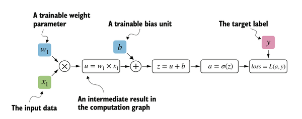
The computation flows like this:

1. Input feature x1 is multiplied by weight w1
2. Bias b is added to get net input z
3. Sigmoid activation function produces output a
4. Loss is computed by comparing output a with target label y

Candle builds such a computation graph in the background, and we can use this to calculate gradients of a loss function with respect to the model parameters (here w1 and b) to train the model.

Note: In the code, we pass z (not a) to binary_cross_entropy_with_logit because this function combines the sigmoid activation and binary cross-entropy loss computation for numerical efficiency. The variable a is computed separately to illustrate the full computation graph as shown in the diagram.

Automatic Differentiation Made Easy

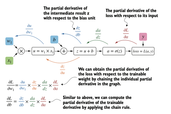
If we carry out computations in Candle, we can build a computational graph to compute gradients. Gradients are required when training neural networks via the popular backpropagation algorithm, which can be considered an implementation of the chain rule from calculus for neural networks.

Partial Derivatives and Gradients

Partial derivatives measure the rate at which a function changes with respect to one of its variables. A gradient is a vector containing all of the partial derivatives of a multivariate function—a function with more than one variable as input.

If you're not familiar with partial derivatives, gradients, or the chain rule from calculus, don't worry. On a high level, all you need to know is that the chain rule is a way to compute gradients of a loss function given the model's parameters in a computation graph. This provides the information needed to update each parameter to minimize the loss function, which serves as a proxy for measuring the model's performance.

Computing Gradients in Candle

How is this related to automatic differentiation? Candle's autograd (automatic differentiation) engine constructs a computational graph by tracking operations performed on Var tensors (variables). Then, by calling .backward(), we can compute the gradients of the loss with respect to the model parameters.

In Candle, we mark tensors that need gradient tracking using the Var type:

use candle_core::{Device, Tensor, Var};
use candle_nn::loss::binary_cross_entropy_with_logit;

fn main() -> Result<(), candle_core::Error> {
    let device = Device::Cpu;

    let y = Tensor::new(&[1.], &device)?;
    let x1 = Tensor::new(&[1.1], &device)?;
    let w1 = Var::new(&[2.2], &device)?;
    let b = Var::new(&[0.], &device)?;

    let z = (&x1 * w1.as_tensor() + b.as_tensor())?;

    let loss = binary_cross_entropy_with_logit(&z, &y.flatten_all()?)?;

    // Backward pass - compute gradients
    let grads = loss.backward()?;

    // Get gradients for our parameters
    let grad_l_w1 = grads.get(&w1);
    let grad_l_b = grads.get(&b);
    println!("{}", grad_l_w1.unwrap());
    println!("{}", grad_l_b.unwrap());

    Ok(())
}

This prints:

[-0.0898]
Tensor[[1], f64]
[-0.0817]
Tensor[[1], f64]

The key differences from regular tensors:

• We create Var instead of Tensor for parameters that need gradients
• We use w1.as_tensor() to get the underlying tensor for computations
• We call loss.backward() to compute all gradients
• We retrieve gradients using grads.get(&variable)

While the calculus concepts may seem overwhelming, all you need to know is that Candle takes care of the calculus for us via the .backward() method—we won't need to compute any derivatives or gradients by hand. Candle automatically tracks operations and computes the necessary gradients for training neural networks.

Implementing Multilayer Neural Networks

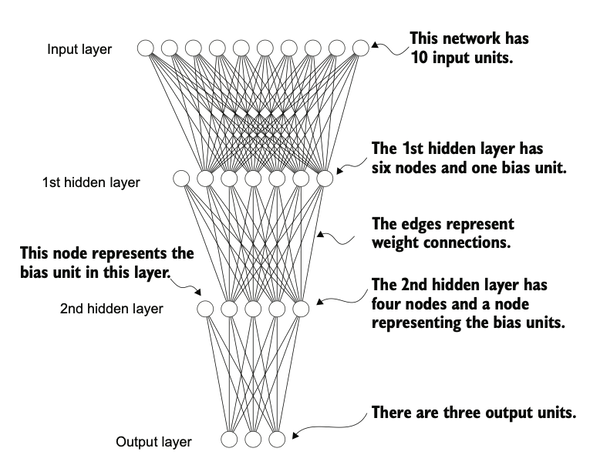
Next, we focus on Candle as a library for implementing deep neural networks. To provide a concrete example, let's look at a multilayer perceptron—a fully connected neural network as illustrated below.

Defining a Neural Network

When implementing a neural network in Candle, we can define a struct to hold our layers and implement the Module trait to specify the forward pass. This approach provides structure and makes it easier to build and train models.

Within our struct, we define the network layers in the new function and specify how the layers interact in the forward method. The forward method describes how the input data passes through the network and comes together as a computation graph. The following code implements a classic multilayer perceptron with two hidden layers:

use candle_core::{Error, Tensor};
use candle_nn::{Linear, Module, VarBuilder, linear};

#[derive(Debug)]
struct NeuralNetwork {
    layer_1: Linear,
    layer_2: Linear,
    output_layer: Linear,
}

impl NeuralNetwork {
    fn new(num_inputs: usize, num_outputs: usize, vb: VarBuilder) -> Result<Self, Error> {
        Ok(Self {
            // 1st hidden layer
            layer_1: linear(num_inputs, 30, vb.pp("l1"))?,
            // 2nd hidden layer
            layer_2: linear(30, 20, vb.pp("l2"))?,
            // output layer
            output_layer: linear(20, num_outputs, vb.pp("out"))?,
        })
    }
}

impl Module for NeuralNetwork {
    fn forward(&self, x: &Tensor) -> Result<Tensor, Error> {
        // Pass through 1st hidden layer with ReLU activation
        let x = self.layer_1.forward(x)?;
        let x = x.relu()?;

        // Pass through 2nd hidden layer with ReLU activation
        let x = self.layer_2.forward(&x)?;
        let x = x.relu()?;

        // Output layer (logits)
        self.output_layer.forward(&x)
    }
}

Coding the number of inputs and outputs as variables allows us to reuse the same code for datasets with different numbers of features and classes. The linear function creates a fully connected layer that takes the number of input and output nodes as arguments. Nonlinear activation functions (ReLU) are placed between the hidden layers.

Creating a Model Instance

We can instantiate a new neural network object as follows:

use candle_core::{DType, Device};
use candle_nn::{VarBuilder, VarMap};

fn main() -> Result<(), candle_core::Error> {
    let device = Device::Cpu;
    let varmap = VarMap::new();
    let vb = VarBuilder::from_varmap(&varmap, DType::F32, &device);

    let model = NeuralNetwork::new(50, 3, vb)?;

    Ok(())
}

Before using this model, we can print it to see its structure:

println!("{:#?}", model);

This prints something like:

NeuralNetwork {
    layer_1: Linear { ... },
    layer_2: Linear { ... },
    output_layer: Linear { ... }
}

Counting Trainable Parameters

Next, let's check the total number of trainable parameters in this model:

fn num_trainable_params(varmap: &VarMap) -> usize {
    let mut total_params = 0;

    for var in varmap.all_vars().iter() {
        let tensor = var.as_tensor();
        total_params += tensor.elem_count();
    }

    total_params
}

println!(
    "Total number of trainable model parameters: {}",
    num_trainable_params(&varmap)
);

This prints:

Total number of trainable model parameters: 2213

Each parameter in the VarMap is trainable and will be updated during training.

Inspecting Layer Weights

In our neural network model, the trainable parameters are contained in the Linear layers. A Linear layer multiplies the inputs with a weight matrix and adds a bias vector. This is sometimes referred to as a feedforward or fully connected layer.

We can access the weight parameter matrix of the first layer:

println!("{}", model.layer_1.weight());

This prints:

[[-0.2709,  0.1136, -0.2754, ...,  0.2414, -0.0017,  0.2840],
 [-0.0263,  0.0686,  0.5760, ...,  0.3354,  0.1075,  0.0547],
 [-0.2206,  0.0207, -0.2632, ..., -0.0896,  0.2400, -0.1271],
 ...
 [-0.1658, -0.1832, -0.2016, ...,  0.0093, -0.0543,  0.3168],
 [-0.1934, -0.1501,  0.1322, ..., -0.2806, -0.2028, -0.0779],
 [ 0.3975,  0.0921, -0.0050, ...,  0.1652,  0.1653,  0.1574]]
Tensor[[30, 50], f32]

Let's check its dimensions:

println!("{:?}", model.layer_1.weight().shape());

The result is:

[30, 50]

The weight matrix is a 30 × 50 matrix. These weights are initialized with small random numbers, which differ each time we instantiate the network. In deep learning, initializing model weights with small random numbers is desired to break symmetry during training. Otherwise, the nodes would perform the same operations and updates during backpropagation, which would not allow the network to learn complex mappings.

Using the Model for Forward Pass

Now let's see how the network is used via the forward pass:

let x = Tensor::rand(0f32, 1f32, (1, 50), &device)?;
let output = model.forward(&x)?;
println!("{}", output);

The result is something like:

[[0.4167, 1.0375, 0.6351]]
Tensor[[1, 3], f32]

We generated a single random training example as a toy input (note that our network expects 50-dimensional feature vectors) and fed it to the model, returning three scores.

The forward pass refers to calculating output tensors from input tensors. This involves passing the input data through all the neural network layers, starting from the input layer, through hidden layers, and finally to the output layer.

Converting Logits to Probabilities

In Candle, it's common practice to code models such that they return the outputs of the last layer (logits) without passing them to a nonlinear activation function. That's because loss functions combine the softmax (or sigmoid for binary classification) operation with the loss computation in a single operation for numerical efficiency.

If we want to compute class-membership probabilities for our predictions, we call the softmax function explicitly:

use candle_nn::ops::softmax;

let output = model.forward(&x)?;
let probabilities = softmax(&output, 1)?;
println!("{}", probabilities);

This prints something like:

Tensor[[0.3113, 0.3934, 0.2952]]

The values can now be interpreted as class-membership probabilities that sum up to 1. The values are roughly equal for this random input, which is expected for a randomly initialized model without training.

Setting Up Data Loaders

Before we can train our model, we need to set up data loaders to iterate over our dataset during training. The overall idea is to create a Dataset that holds our data, then create a DataLoader that samples batches from it.

Creating a Toy Dataset

Let's start by creating a simple toy dataset of five training examples with two features each. We also create labels for these examples: three belong to class 0, and two belong to class 1. In addition, we make a test set consisting of two entries:

use candle_core::{DType, Device, Error, Tensor};

fn main() -> Result<(), Error> {
    let device = Device::Cpu;

    let x_train = Tensor::new(
        &[
            [-1.2, 3.1],
            [-0.9, 2.9],
            [-0.5, 2.6],
            [2.3, -1.1],
            [2.7, -1.5],
        ],
        &device,
    )?
    .to_dtype(DType::F32)?;
    let y_train = Tensor::new(&[0., 0., 0., 1., 1.], &device)?.to_dtype(DType::U32)?;
    let x_test = Tensor::new(&[[-0.8, 2.8], [2.6, -1.6]], &device)?.to_dtype(DType::F32)?;
    let y_test = Tensor::new(&[0., 1.], &device)?.to_dtype(DType::U32)?;

    Ok(())
}

Note that class labels should start with 0, and the largest class label value should not exceed the number of output nodes minus 1. So if we have class labels 0, 1, 2, 3, and 4, the neural network output layer should consist of five nodes.

Defining a Dataset Struct

Next, we create a custom Dataset struct to hold our data:

struct Dataset {
    features: Tensor,
    labels: Tensor,
}

impl Dataset {
    fn new(x: Tensor, y: Tensor) -> Self {
        Self {
            features: x,
            labels: y,
        }
    }

    fn get_item(&self, index: usize) -> Result<(Tensor, Tensor), Error> {
        let one_x = self.features.get(index)?;
        let one_y = self.labels.get(index)?;
        Ok((one_x, one_y))
    }

    fn len(&self) -> Result<usize, Error> {
        self.labels.dims1()
    }
}

Let's create training and testing datasets:

// We clone the tensors because Dataset::new takes ownership.
// This keeps the originals available if needed later.
// For large datasets, consider using references to avoid cloning overhead.
let train_ds = Dataset::new(x_train.clone(), y_train.clone());
let test_ds = Dataset::new(x_test.clone(), y_test.clone());

The main components of our Dataset are:

• new method that sets up the features and labels
• get_item method that returns exactly one data record and its label via an index
• len method that returns the total length of the dataset

We can verify the length:

println!("{}", train_ds.len()?); // Prints: 5

Creating a DataLoader

Now we create a DataLoader that samples batches from our dataset. In Rust, we implement this using the Iterator trait, which allows us to create batches on-demand rather than pre-computing all batches upfront.

use rand::seq::SliceRandom;

struct DataLoader {
    dataset: Dataset,
    batch_size: usize,
    indices: Vec<usize>,
    drop_last: bool,
}

impl DataLoader {
    fn new(
        dataset: Dataset,
        batch_size: usize,
        shuffle: bool,
        drop_last: bool,
    ) -> Result<Self, Error> {
        let len = dataset.len()?;
        let mut indices: Vec<usize> = (0..len).collect();

        if shuffle {
            indices.shuffle(&mut rand::rng());
        }

        Ok(Self {
            dataset,
            batch_size,
            indices,
            drop_last,
        })
    }

    fn iter(&self) -> DataLoaderIter {
        DataLoaderIter {
            dataset: &self.dataset,
            indices: &self.indices,
            batch_size: self.batch_size,
            drop_last: self.drop_last,
            current: 0,
        }
    }

    fn total_batches(&self) -> usize {
        if self.drop_last {
            self.indices.len() / self.batch_size
        } else {
            (self.indices.len() + self.batch_size - 1) / self.batch_size
        }
    }
}

struct DataLoaderIter<'a> {
    dataset: &'a Dataset,
    indices: &'a [usize],
    batch_size: usize,
    drop_last: bool,
    current: usize,
}

impl<'a> Iterator for DataLoaderIter<'a> {
    type Item = Result<(Tensor, Tensor), Error>;

    fn next(&mut self) -> Option<Self::Item> {
        if self.current >= self.indices.len() {
            return None;
        }

        let end = (self.current + self.batch_size).min(self.indices.len());
        let batch_indices = &self.indices[self.current..end];

        // Drop last incomplete batch if specified
        if self.drop_last && batch_indices.len() < self.batch_size {
            return None;
        }

        self.current = end;

        let mut batch_features = Vec::new();
        let mut batch_labels = Vec::new();

        for &idx in batch_indices {
            match self.dataset.get_item(idx) {
                Ok((features, labels)) => {
                    batch_features.push(features);
                    batch_labels.push(labels);
                }
                Err(e) => return Some(Err(e)),
            }
        }

        match (
            Tensor::stack(&batch_features, 0),
            Tensor::stack(&batch_labels, 0),
        ) {
            (Ok(batch_x), Ok(batch_y)) => Some(Ok((batch_x, batch_y))),
            (Err(e), _) | (_, Err(e)) => Some(Err(e)),
        }
    }
}

Let's create data loaders for training and testing:

let train_loader = DataLoader::new(train_ds, 2, true, true)?;
let test_loader = DataLoader::new(test_ds, 2, false, true)?;

The parameters are:

• batch_size: How many examples per batch
• shuffle: Whether to shuffle the data (useful for training)
• drop_last: Whether to drop the last incomplete batch

Iterating Over Batches

We can iterate over the data loader:

for (idx, batch_result) in train_loader.iter().enumerate() {
    let (x, y) = batch_result?;
    println!("Batch {}: {}  {}", idx + 1, x, y);
}

The result is:

Batch 1: [[-0.9000,  2.9000],
 [-0.5000,  2.6000]]
Tensor[[2, 2], f32]  [0, 0]
Tensor[[2], u32]
Batch 2: [[ 2.3000, -1.1000],
 [-1.2000,  3.1000]]
Tensor[[2, 2], f32]  [1, 0]
Tensor[[2], u32]

The data loader iterates over the training dataset, visiting each training example exactly once. This is known as a training epoch. Since we set shuffle=true, the order of examples will be different each time we create a new data loader.

Why Drop Last Batch?

We specified a batch size of 2, but if we had set drop_last=false, the last batch might contain only one example (since 5 is not evenly divisible by 2). Having a substantially smaller batch as the last batch in a training epoch can disturb convergence during training. Setting drop_last=true prevents this by omitting the incomplete last batch.

Building From Scratch

Unlike PyTorch, which has built-in Dataset and DataLoader classes, we built these from scratch in Candle. This gives us more control and helps understand what's happening under the hood. The core concepts remain the same:

• A dataset holds data and provides individual items
• A data loader batches items together and handles shuffling
• We iterate through batches during training

A Typical Training Loop

Let's now train a neural network on our toy dataset. The following code shows the training loop:

use candle_nn::{Optimizer, SGD};
use candle_nn::loss::cross_entropy;

let varmap = VarMap::new();
let vb = VarBuilder::from_varmap(&varmap, DType::F32, &device);

// The dataset has two features and two classes
let model = NeuralNetwork::new(2, 2, vb)?;

// Create optimizer with learning rate 0.5
let mut optimizer = SGD::new(varmap.all_vars(), 0.5)?;

let num_epochs = 3;
for epoch in 0..num_epochs {
    for (batch_idx, batch_result) in train_loader.iter().enumerate() {
        let (features, labels) = batch_result?;

        // Forward pass
        let logits = model.forward(&features)?;
        let loss = cross_entropy(&logits, &labels)?;

        // Backward pass and parameter update
        optimizer.backward_step(&loss)?;

        // Logging
        let loss_val = loss.to_vec0::<f32>()?;
        println!(
            "Epoch: {:03}/{:03} | Batch {:03}/{:03} | Train Loss: {:.2}",
            epoch + 1,
            num_epochs,
            batch_idx + 1,
            train_loader.total_batches(),
            loss_val
        );
    }
}

Running this code yields output like:

Epoch: 001/003 | Batch 001/002 | Train Loss: 3.64
Epoch: 001/003 | Batch 002/002 | Train Loss: 0.00
Epoch: 002/003 | Batch 001/002 | Train Loss: 3.33
Epoch: 002/003 | Batch 002/002 | Train Loss: 0.00
Epoch: 003/003 | Batch 001/002 | Train Loss: 0.00
Epoch: 003/003 | Batch 002/002 | Train Loss: 0.00

As we can see, the loss reaches near 0 after three epochs, a sign that the model converged on the training set.

Understanding the Training Process

Here, we initialize a model with two inputs and two outputs because our toy dataset has two input features and two class labels to predict. We use a stochastic gradient descent (SGD) optimizer with a learning rate of 0.5.

The learning rate is a hyperparameter—a tunable setting we must experiment with based on observing the loss. Ideally, we want to choose a learning rate such that the loss converges after a certain number of epochs. The number of epochs is another hyperparameter to choose.

As discussed earlier, we pass the logits directly into the cross_entropy loss function, which applies the softmax function internally for numerical efficiency. In Candle, optimizer.backward_step(&loss) does both the gradient computation and the parameter update in one call, which is convenient.

Making Predictions

After training the model, we can use it to make predictions:

let outputs = model.forward(&x_train)?;
println!("{}", outputs);

The results might look like:

[[  4.7010e1,  -3.7848e1],
 [  4.2802e1,  -3.4469e1],
 [  3.7059e1,  -2.9854e1],
 [ -6.4291e0, -3.9145e-1],
 [ -8.2538e0,  3.6420e-2]]
Tensor[[5, 2], f32]

Converting to Probabilities

To obtain the class membership probabilities, we use the softmax function:

use candle_nn::ops::softmax;

let probas = softmax(&outputs, 1)?;
println!("{}", probas);

This outputs something like:

[[  1.0000e0, 1.4011e-37],
 [  1.0000e0, 2.7653e-34],
 [  1.0000e0, 8.7143e-30],
 [ 2.3815e-3,  9.9762e-1],
 [ 2.5089e-4,  9.9975e-1]]
Tensor[[5, 2], f32]

Looking at the first row, the first value means the training example has a 99.91% probability of belonging to class 0 and a 0.09% probability of belonging to class 1.

Getting Class Labels

We can convert these values into class label predictions using the argmax function, which returns the index position of the highest value in each row:

let predictions = probas.argmax(1)?;
println!("predictions: {}", predictions);

This prints:

[0, 0, 0, 1, 1]
Tensor[[5], u32]

Note that it's unnecessary to compute softmax probabilities to obtain the class labels. We can apply argmax to the logits directly:

let predictions = outputs.argmax(1)?;
println!("predictions: {}", predictions);

The output is the same:

[0, 0, 0, 1, 1]
Tensor[[5], u32]

Computing Accuracy

We can check if our predictions match the true labels:

println!("{}", predictions.eq(&y_train)?.sum_all()?);

This outputs:

[5]
Tensor[[], u8]

Since the dataset consists of five training examples, we have five out of five predictions correct, which is 5/5 × 100% = 100% prediction accuracy.

To generalize the computation of prediction accuracy, let's implement a function:

fn compute_accuracy(model: &NeuralNetwork, dataloader: &DataLoader) -> Result<f32, Error> {
    let mut correct = 0;
    let mut total_examples = 0;

    for batch_result in dataloader.iter() {
        let (features, labels) = batch_result?;

        let logits = model.forward(&features)?;
        let predictions = logits.argmax(1)?;

        // Returns a tensor of True/False values
        let compare = predictions.eq(&labels)?;

        // Count number of correct predictions
        let correct_batch = compare.sum_all()?;
        // Convert Tensor to u8 value
        correct += correct_batch.to_vec0::<u8>()?;

        total_examples += compare.elem_count();
    }

    Ok(correct as f32 / total_examples as f32)
}

The code iterates over a data loader to compute the number and fraction of correct predictions. This method scales to datasets of arbitrary size since, in each iteration, the dataset chunk that the model receives is the same size as the batch size seen during training.

We can apply the function to the training set:

let accuracy = compute_accuracy(&model, &train_loader)?;
println!("{}", accuracy);

The result is:

1

Similarly, we can apply it to the test set:

let accuracy = compute_accuracy(&model, &test_loader)?;
println!("{}", accuracy);

This prints:

1

Both show 100% accuracy, indicating our model learned the toy dataset perfectly!

Saving and Loading Models

Now that we've trained our model, let's see how to save it so we can reuse it later.

Saving a Model

Candle uses the SafeTensors format for saving models, which is a safe and efficient way to store tensor data:

// Save model
varmap.save("model.safetensors")?;

The varmap is a collection that holds all the model's trainable parameters (weights and biases). "model.safetensors" is the filename for the model file saved to disk. The .safetensors extension is the standard convention for this format.

Loading a Model

Once we've saved the model, we can restore it from disk:

fn main() -> Result<(), candle_core::Error> {
    let device = Device::Cpu;
    let mut varmap_loaded = VarMap::new();
    let vb = VarBuilder::from_varmap(&varmap_loaded, DType::F32, &device);

    // Create new model with same architecture
    let model_loaded = NeuralNetwork::new(2, 2, vb)?;

    // Load the saved parameters
    varmap_loaded.load("model.safetensors")?;

    Ok(())
}

The process works in three steps:

1. Create a new VarMap: We create an empty VarMap to hold the loaded parameters
2. Reconstruct the model architecture: We create a new NeuralNetwork instance with the same architecture (2 inputs, 2 outputs) as the saved model
3. Load the parameters: We call varmap_loaded.load() to read the file and populate the VarMap with the saved weights and biases

The model architecture (here NeuralNetwork::new(2, 2)) needs to match the original saved model exactly. If the architecture doesn't match, the loading will fail because the parameter shapes won't align.

Also note that variable names must match exactly—the layer prefixes like "l1", "l2", and "out" used during model creation must be identical when loading.

Verifying the Loaded Model

We can verify that the loaded model works correctly by computing accuracy:

let accuracy = compute_accuracy(&model_loaded, &train_loader)?;
println!("{}", accuracy);

This should give the same accuracy as before saving, confirming that the model's learned parameters were successfully restored.

Why SafeTensors?

SafeTensors is a modern format designed specifically for safely storing and loading tensor data. It's:

• Fast: Efficient serialization and deserialization
• Safe: Prevents arbitrary code execution during loading
• Portable: Works across different frameworks and languages

This makes it ideal for sharing models and deploying them in production environments.

Conclusion

We've covered the basics of working with Candle—tensor operations, building neural networks, automatic differentiation, and training models. By porting PyTorch examples to Candle, we've seen that the core concepts of deep learning remain the same across frameworks.

While we used a simple toy dataset here, these concepts scale to real-world applications.

The full code is available on GitHub! Happy coding! 😊